Algebra of physical space

Algebra of Physical Space (APS)

Mathematical concepts	Paravector algebra

Applications in Physics	Special Relativity with APS The Dirac equation with APS

In physics, the algebra of physical space (APS) is the use of the Clifford or geometric algebra Cℓ₃ of the three-dimensional Euclidean space as a model for (3+1)-dimensional space-time, representing a point in space-time via a paravector (3-dimensional vector plus a 1-dimensional scalar).

The Clifford algebra Cℓ₃ has a faithful representation, generated by Pauli matrices, on the spin representation C²; further, Cℓ₃ is isomorphic to the even subalgebra of the 3+1 Clifford algebra, Cℓ0
3,1.

APS can be used to construct a compact, unified and geometrical formalism for both classical and quantum mechanics.

APS should not be confused with spacetime algebra (STA), which concerns the Clifford algebra Cℓ_1,3(R) of the four dimensional Minkowski spacetime.

1 Special Relativity
2 Classical Electrodynamics
3 Relativistic Quantum Mechanics
4 Classical Spinor
5 See also
6 References
- 6.1 Textbooks
- 6.2 Articles

Special Relativity

In APS, the space-time position is represented as a paravector

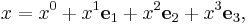
$x = x^0 %2B x^1 \mathbf{e}_1 %2B x^2 \mathbf{e}_2 %2B x^3 \mathbf{e}_3,$

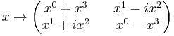
where the time is given by the scalar part $t=x^0$ with $c=1$ . In the Pauli matrix representation the unit basis vectors are replaced by the Pauli matrices and the scalar part by the identity matrix. This means that the Pauli matrix representation of the space-time position is

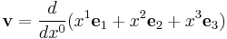
$x \rightarrow \begin{pmatrix} x^0 %2B x^3 && x^1 - ix^2 \\ x^1 %2B ix^2 && x^0-x^3 \end{pmatrix}$

The four-velocity also called proper velocity is paravector defined as the proper time derivative of the space-time position

$u = \frac{d x }{d \tau} = \frac{d x^0}{d\tau} %2B \frac{d}{d\tau}(x^1 \mathbf{e}_1 %2B x^2 \mathbf{e}_2 %2B x^3 \mathbf{e}_3) = \frac{d x^0}{d\tau}(1 %2B \frac{d}{d x^0}(x^1 \mathbf{e}_1 %2B x^2 \mathbf{e}_2 %2B x^3 \mathbf{e}_3)).$

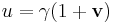
This expression can be brought to a more compact form by defining the ordinary velocity as

$\mathbf{v} = \frac{d}{d x^0}(x^1 \mathbf{e}_1 %2B x^2 \mathbf{e}_2 %2B x^3 \mathbf{e}_3)$

and recalling the definition of the gamma factor, so that the proper velocity becomes

$u = \gamma(1%2B \mathbf{v})$

The proper velocity is a positive unimodular paravector, which implies the following condition in terms of the Clifford conjugation

$u \bar{u} = 1$

The proper velocity transforms under the action of the Lorentz rotor $L$ as

$u \rightarrow u^\prime = L u L^\dagger.$

The restricted Lorentz transformations that preserve the direction of time and include rotations and boosts can be performed by an exponentiation of the space-time rotation biparavector $W$

$L = e^{\frac{1}{2}W}$

In the matrix representation the Lorentz rotor is seen to form an instance of the SL(2,C) group, which is the double cover of the Lorentz group. The unimodularity of the Lorentz rotor is translated in the following condition in terms of the product of the Lorentz rotor with its Clifford conjugation

$L\bar{L} = \bar{L} L = 1$

This Lorentz rotor can be always decomposed in two factors, one Hermitian $B=B^{\dagger}$ , and the other unitary $R^{\dagger}=R^{-1}$ , such that

$L = B R^{\,}$

The unitary element $R$ is called rotor because encodes rotations and the Hermitian element $B$ is called boost.

The four-momentum in APS can be obtained by multiplying the proper velocity with the mass as

$p = m u^{\,},$

with the mass shell condition translated into

$\bar{p}p = m^2$

Classical Electrodynamics

The electromagnetic field is represented as a bi-paravector $F$ , with the Hermitian part representing the Electric field and the anti-Hermitian part representing the magnetic field. In the standard Pauli matrix representation, the electromagnetic field is

$F = \mathbf{E}%2B i \mathbf{B} \rightarrow \begin{pmatrix} E_3 & E_1 -i E_2 \\ E_1 %2Bi E_2 & -E_3 \end{pmatrix} %2B i \begin{pmatrix} B_3 & B_1 -i B_2 \\ B_1 %2Bi B_2 & -B_3 \end{pmatrix}$

The electromagnetic field is obtained from the paravector potential $A=\phi%2B\mathbf{A}$ as

$F = \langle \partial \bar{A} \rangle_V.$

and the electromagnetic field is invariant under a gauge transformation of the form

$A \rightarrow A %2B \partial \chi,$

where $\chi$ is a scalar function.

The Electromagnetic field is covariant under Lorentz transformations according to the law

$F \rightarrow F^\prime = L F \bar{L}$

The Maxwell equations can be expressed in a single equation as follows

$\bar{\partial} F = \frac{1}{ \epsilon} \bar{j},$

where the overbar represents the Clifford conjugation and the four-current is defined as

$j = \rho %2B \mathbf{j}.$

The electromagnetic Lagrangian is

$L = \frac{1}{2} \langle F F \rangle_S - \langle A \bar{j} \rangle_S,$

which is evidently a real scalar invariant.

The Lorentz force equation takes the form

$\frac{d p}{d \tau} = e \langle F u \rangle_{R}$

Relativistic Quantum Mechanics

The Dirac equation takes the form

$i \bar{\partial} \Psi\mathbf{e}_3 %2B e \bar{A} \Psi = m \bar{\Psi}^\dagger$ ,

where $\mathbf{e}_3$ is an arbitrary unitary vector and $A$ is the paravector potential that includes the vector potential and the electric potential.

Classical Spinor

The differential equation of the Lorentz rotor that is consistent with the Lorentz force is

$\frac{d \Lambda}{ d \tau} = \frac{e}{2mc} F \Lambda,$

such that the proper velocity is calculated as the Lorentz transformation of the proper velocity at rest

$u = \Lambda \Lambda^\dagger,$

which can be integrated to find the space-time trajectory $x(\tau)$ with the additional use of

$\frac{d x}{ d \tau} = u$

References

Textbooks

Baylis, William (2002). Electrodynamics: A Modern Geometric Approach (2nd ed.). Birkhäuser. ISBN 0-8176-4025-8
W. E. Baylis, editor, Clifford (Geometric) Algebra with Applications to Physics, Mathematics, and Engineering, Birkhäuser, Boston 1996.
Chris Doran and Anthony Lasenby, Geometric Algebra for Physicists, Cambridge University Press (2003)
David Hestenes: New Foundations for Classical Mechanics (Second Edition). ISBN 0-7923-5514-8, Kluwer Academic Publishers (1999)

Articles

Baylis, William (2002). Relativity in Introductory Physics, Can. J. Phys. 82 (11), 853—873 (2004). (ArXiv:physics/0406158)
W. E. Baylis and G. Jones, The Pauli-Algebra Approach to Special Relativity, J. Phys. A22, 1-16 (1989)
W. E. Baylis, Classical eigenspinors and the Dirac equation ,Phys Rev. A, Vol 45, number 7 (1992)
W. E. Baylis, Relativistic dynamics of charges in electromagnetic fields: An eigenspinor approach ,Phys Rev. A, Vol 60, number 2 (1999)